Introduction to Pharmacokinetics

An understanding of the characteristics of drug exposure following administration and how it relates to safety and efficacy is critical for progressing drug development (e.g. in decision making for drug candidates, design of dosing regimens and making predictions for future studies) as well as being a requirement for regulatory authorities. Pharmacokinetics (PK) analysis aims to evaluate quantitatively how a drug enters the body, what happens to the drug while in the body and ultimately, how it is removed. These processes are commonly referred to by the acronym ‘ADME’, which comprises absorption, distribution, metabolism and excretion.

Non-compartmental analysis (NCA) is a rapid and cost effective method ideally suited to estimating exposure from bioanalytical concentration data. Our team at Drug Development Solutions (DDS) specialises in NCA and has performed hundreds of analyses ranging from small dose range findings studies, regulated toxicology studies and clinical studies (including first in human through to phase III trials). NCA provides critical information such as:

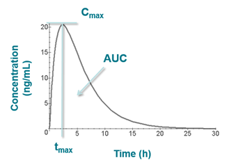
• Maximum plasma concentration attained following dose administration (C_max)
• Time at which the maximum concentration was reached (t_max)
• The area under the plasma concentration vs time curve (AUC)
• Clearance (a total measure of the various mechanisms by which the body removes drug, expressed as volume of blood from which all drug is removed per unit time)
• Volume of distribution (a measure of the extent to which drug distributes out of the blood and into other tissues; a theoretical volume)
• Half-life (time taken for concentration of drug to fall by half)
• Renal clearance
• Amount of drug (and / or metabolite) excreted into urine or faeces
• Fraction of dose excreted in urine or faeces

Parameter values also allow us to evaluate the relationship between dose and exposure, bioavailability, the extent of accumulation of drug with repeated administration, formulation differences and variation in exposure between the sexes etc.

The illustration below (which follows extravascular administration) shows C_max and t_max on a plot of concentration vs time as well as the area under the curve (AUC).

Read more details on specific methods of AUC calculation

More on clearance, volume and half-life

An algebraic equation can be represented graphically on an x/y plot (for example, the equation of a straight line can be represented graphically, given initial values for slope and intercept). Conversely, an equation can be chosen to fit real life data.

The simplest pharmacokinetic scenario is one where the drug is administered intravenously into a single theoretical compartment. In this model, drug is assumed to mix/disperse instantaneously within the compartment. Concentration data for this theoretical compartment are derived from samples of blood, however it is important to note that the compartment may comprise other physiological areas into which drug disperses, such as highly perfused tissue (heart, liver, kidney etc.). However, the dispersal is instantaneous, and because drug levels are therefore homogenous across the blood and these tissues, the measurements taken from the blood following administration are assumed to be representative of the compartment as a whole. These measurements can be plotted as follows:

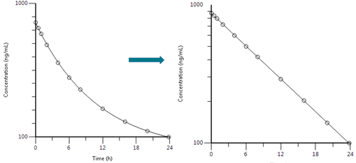
Most drugs follow first order elimination with logarithmic declines in concentration governed by a rate constant often referred to as the elimination rate constant, 𝝺z or Kel where Kel is the gradient of the line in the plots above.

The model can be represented pictorially: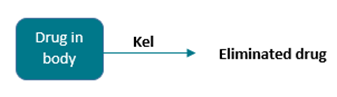

Bioanalytical data is a best estimate to which an equation can be fitted. In the above case of IV administration followed by first order elimination (and no distribution phase) the decline in concentration can best be described by the following equation:

LnC = - kel t + LnC_o

or

C = C_o e ^{kel t}

where C = concentration at time t; C₀ = y intercept at t0 (initial concentration); kel = gradient.

This equation can be rearranged to derive an equation for half-life (t_1/2, the time taken for concentration to fall by half, or to achieve 0.5*C₀):

t_1/2=In(0.5) / kel

The change in drug concentration in this single theoretical compartment may be described by values such as AUC, C_max and half-life, but it is driven by physiology i.e. the volume of the ‘container’ (volume of distribution), and the ability of the body to remove drug (total clearance, which refers to the sum of clearance mechanisms (renal clearance + hepatic clearance… etc.).

Clearance is calculated by CL = Dose / AUC_^0-inf
Volume is calculated by V = CL / kel
Therefore the equation of the line can also be written as:

C = C_o e^{- CL/Vt}

Note that clearance and volume require the total amount of drug that enters systemic circulation to be known. This applies after IV administration. Following extravascular administration not all of the drug will enter systemic circulation and therefore parameters are denoted CL/F and Vz/F to indicate that values are subject to bioavailability being accounted for. Where the dose administered is an amount per unit of bodyweight (e.g. 1 mg/kg), body weight of each individual subject must be factored into the calculation. Alternatively, units may be expressed per unit of body weight, e.g. L/h/kg.

Clearance and volume determine the slope of the line, and the slope of the line determines exposure of the drug, half-life etc. Clearance and volume are therefore termed primary pharmacokinetic parameters.

Note that renal clearance may be estimated following urine analysis. Please click here for more information.

In the model described above, drug may have distributed from the plasma into other highly perfused tissues, but this movement was instantaneous, reversible and at equilibrium. However it may be that drug distributes into other tissues such as muscle and other organs.

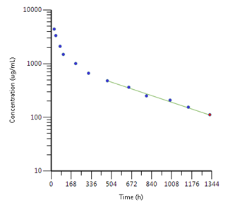
In a two compartment IV model, there may be an initial ‘fast phase’ or faster decline in concentrations due to the initial net movement of drug from the blood (or ‘central’ compartment) into these other tissues. Once equilibrium is reached, the decline is known as the terminal elimination phase. Half-life is measured from a regression line fitted to this phase, and is therefore termed ‘terminal elimination half-life’. The slope of the line (Kel) is used to calculate volume of distribution and for extrapolation in calculation of AUC_0-inf.
An example is shown below:

This can be represented pictorially:

In NCA, the equation C = C_o e^{- kel t} is fitted to the terminal elimination phase in order to derive parameters. The criteria used at DDS to determine acceptability of the regression line are set out clearly in our study plans. Additionally, we are always happy to give you the opportunity to review the regression lines used to calculate terminal elimination half-life. More complex equations may be fitted to describe the entire concentration vs time curve, however this is beyond the scope of NCA and is not described here.
This guide serves as a basic overview of the typical calculations performed at DDS. For further information or to speak to one of our pharmacokineticists please contact us.